Chapter 13 Data Wrangling
So far in our journey, we’ve seen how to look at data saved in data frames using the glimpse() and View() functions in Chapter 11 on and how to create data visualizations using the ggplot2 package in Chapter 12. In particular we studied what we term the the following three graphs:
- scatterplots via
geom_point() - histograms via
geom_histogram() - barplots via
geom_bar()orgeom_col()
We created these visualizations using the “Grammar of Graphics”, which maps variables in a data frame to the aesthetic attributes of one the above 3 geometric objects. We can also control other aesthetic attributes of the geometric objects such as the size and color as seen in the Gapminder data example in Figure 12.1.
Recall however in previous chapters we discussed that for two of our visualizations we needed transformed/modified versions of existing data frames. Recall for example the scatterplot of economic mobility only for neighborhoods in Wisconsin. In order to create this visualization, we needed to first pare down the atlas data frame to a new data frame atlas_wisconsin. consisting of only state == 55 neighborhoods using the filter() function.
atlas_wisconsin <- atlas %>%
  filter(state == 55)

ggplot(data = atlas_wisconsin, mapping = aes(x = med_hhinc2016, y = kfr_pooled_p25)) +
  geom_point()
In this chapter, we’ll introduce two very useful functions from the dplyr package that will allow you to take a data frame and
filter()its existing rows to only pick out a subset of them. For example, theatlas_wisconsindata frame above.mutate()its existing columns/variables to create new ones. For example, convert dollars to log dollars.
There are other functions we will not cover here, but that could be really useful for you to know if you ever get to work with data outside this course: summarize(), group_by(), arrange() and join(). I will leave those to learn on your own if you want to. You can check this very good explanation.
Back to our functions! Notice how we used computer code font to describe the actions we want to take on our data frames. This is because the dplyr package for data wrangling that we’ll introduce in this chapter has intuitively verb-named functions that are easy to remember.
We’ll start by introducing the pipe operator %>%, which allows you to combine multiple data wrangling verb-named functions into a single sequential chain of actions.
Needed packages
Let’s load all the packages needed for this chapter (this assumes you’ve already installed them). If needed, read Section 11.6 for information on how to install and load R packages. We will also load the atlas data once more.
library(dplyr)
library(ggplot2)
atlas <- readRDS(gzcon(url("https://raw.githubusercontent.com/jrm87/ECO3253_repo/master/data/atlas.rds")))
13.1 The pipe operator: %>%
Before we start data wrangling, let’s first introduce a very nifty tool that gets loaded along with the dplyr package: the pipe operator %>%. Say you would like to perform a hypothetical sequence of operations on a hypothetical data frame x using hypothetical functions f(), g(), and h():
- Take
xthen - Use
xas an input to a functionf()then - Use the output of
f(x)as an input to a functiong()then - Use the output of
g(f(x))as an input to a functionh()
One way to achieve this sequence of operations is by using nesting parentheses as follows:
The above code isn’t so hard to read since we are applying only three functions: f(), then g(), then h(). However, you can imagine that this can get progressively harder and harder to read as the number of functions applied in your sequence increases. This is where the pipe operator %>% comes in handy. %>% takes one output of one function and then “pipes” it to be the input of the next function. Furthermore, a helpful trick is to read %>% as “then.” For example, you can obtain the same output as the above sequence of operations as follows:
You would read this above sequence as:
- Take
xthen - Use this output as the input to the next function
f()then - Use this output as the input to the next function
g()then - Use this output as the input to the next function
h()
So while both approaches above would achieve the same goal, the latter is much more human-readable because you can read the sequence of operations line-by-line. But what are the hypothetical x, f(), g(), and h()? Throughout this chapter on data wrangling:
- The starting value
xwill be a data frame. For example:atlas. - The sequence of functions, here
f(),g(), andh(), will be a sequence of any number of the 6 data wrangling verb-named functions we listed in the introduction to this chapter. For example:filter(state == 55). - The result will be the transformed/modified data frame that you want. For example: a data frame consisting of only the subset of rows in
atlascorresponding to neighborhoods in the State of Wisconsin.
Much like when adding layers to a ggplot() using the + sign at the end of lines, you form a single chain of data wrangling operations by combining verb-named functions into a single sequence with pipe operators %>% at the end of lines. So continuing our example involving neighborhoods in Wisconsin, we form a chain using the pipe operator %>% and save the resulting data frame in atlas_wisconsin:
Keep in mind, there are many more advanced data wrangling functions than just the 2 listed in the introduction to this chapter; you’ll see some examples of these in Section 13.4. However, just with these 2 verb-named functions you’ll be able to perform a broad array of data wrangling tasks for the rest of this course.
13.2 filter rows
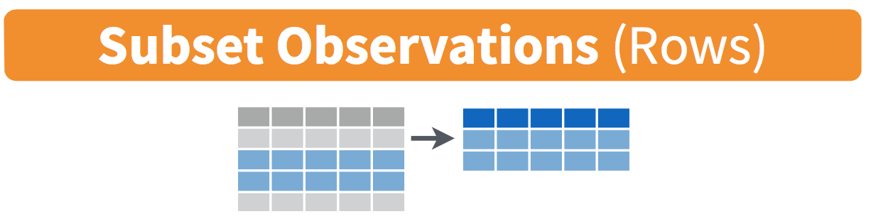
Figure 13.1: Diagram of
The filter() function here works much like the “Filter” option in Microsoft Excel; it allows you to specify criteria about the values of a variable in your dataset and then filters out only those rows that match that criteria. We begin by focusing only on neighborhoods from the state of North Carolina. The state code (or airport code) for Portland, Oregon is 37. Run the following and look at the resulting spreadsheet to ensure that only neighborhoods from North Carolina are chosen here:
Note the following:
- The ordering of the commands:
- Take the
atlasdata frame then filterthe data frame so that only thosewithstateequals37are included.
- Take the
- We test for equality using the double equal sign
==and not a single equal sign=. In other wordsfilter(state = 37)will yield an error. This is a convention across many programming languages. If you are new to coding, you’ll probably forget to use the double equal sign==a few times before you get the hang of it.
You can use other mathematical operations beyond just == to form criteria:
>corresponds to “greater than”<corresponds to “less than”>=corresponds to “greater than or equal to”<=corresponds to “less than or equal to”!=corresponds to “not equal to”. The!is used in many programming languages to indicate “not”.
Furthermore, you can combine multiple criteria together using operators that make comparisons:
|corresponds to “or”&corresponds to “and”
To see many of these in action, let’s filter atlas for all rows that:
- Had a mean household income over 30,000 in the year 2000 and
- Are in North Carolina or Massachusetts; and
- Had an employment rate in the year 2000 of at least 80%
Run the following:
atlas_filter1 <- atlas %>%
  filter(hhinc_mean2000 >30000 & (state ==37  | state == 25) & emp2000 >= 0.8)
View(atlas_filter1)
Note that even though colloquially speaking one might say “all neighborhoods from North Carolina and Massachusetts” in terms of computer operations, we really mean “all neighborhoods from North Carolina or Massachusetts.” For a given row in the data, state can be 37, 25, or something else, but not 37 and 25 at the same time. Furthermore, note the careful use of parentheses around the state ==37 | state == 25.
We can often skip the use of & and just separate our conditions with a comma. In other words the code above will return the identical output atlas_filter1 as this code below:
atlas_filter1 <- atlas %>%
  filter(hhinc_mean2000 >30000, (state ==37  | state == 25), emp2000 >= 0.8)
View(atlas_filter1)
Let’s present another example that uses the ! “not” operator to pick rows that don’t match a criteria. As mentioned earlier, the ! can be read as “not.” Here we are filtering rows corresponding to neighborhoods that are not in North Carolina or Massachusetts.
Again, note the careful use of parentheses around the (state ==37 | state == 25). If we didn’t use parentheses as follows:
We would be returning all neighborhoods not in 37 or those in 25, which is an entirely different resulting data frame.
Now say we have a large list of airports we want to filter for, say NC (37), MA (25), FL(12) and PA(42). We could continue to use the | or operator as so:
atlas_many_states <- atlas %>%
  filter(state ==37  | state == 25 | state == 12 | state == 42)
View(atlas_many_states)
but as we progressively include more airports, this will get unwieldy. A slightly shorter approach uses the %in% operator:
What this code is doing is filtering atlas for all neighborhoods where state is in the list of airports c(37, 25, 12, 42). Recall from Chapter 11 that the c() function “combines” or “concatenates” values in a vector of values. Both outputs of atlas_many_states are the same, but as you can see the latter takes much less time to code.
As a final note we point out that filter() should often be among the first verbs you apply to your data. This cleans your dataset to only those rows you care about, or put differently, it narrows down the scope of your data frame to just the observations your care about.
13.3 mutate existing variables
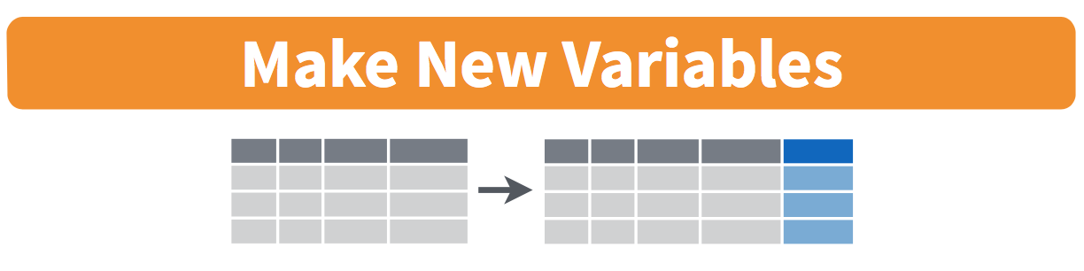
Figure 13.2: Mutate diagram from Data Wrangling with dplyr and tidyr cheatsheet
A common transformation of data is to create/compute new variables based on existing ones. For example, say you are more comfortable thinking of income in terms of the logarithm of income instead of in dollars. We will apply this to the variable hhinc_mean2000 (the mean household income in 2000). You want to implement the following formula:
\[ \text{income} = log(\text{income}) \]
We can apply this formula to the hhinc_mean2000 variable using the mutate() function, which takes existing variables and mutates them to create new ones.
Note that we have overwritten the original atlas data frame with a new version that now includes the additional variable log_hhinc_mean2000. In other words, the mutate() command outputs a new data frame which then gets saved over the original atlas data frame. Furthermore, note how in mutate() we used log_hhinc_mean2000= log(hhinc_mean2000) to create a new variable log_hhinc_mean2000.
Why did we overwrite the data frame atlas instead of assigning the result to a new data frame like atlas_new, but on the other hand why did we not overwrite hhinc_mean2000, but instead created a new variable called temp_in_C? As a rough rule of thumb, as long as you are not losing original information that you might need later, it’s acceptable practice to overwrite existing data frames. On the other hand, had we used mutate(hhinc_mean2000 = log(hhinc_mean2000) instead of mutate(log_hhinc_mean2000= log(hhinc_mean2000)), we would have overwritten the original variable hhinc_mean2000 and lost its values.
13.4 Other verbs
Here are some other useful data wrangling verbs that might come in handy:
select()only a subset of variables/columnsrename()variables/columns to have new names- Return only the
top_n()values of a variable
13.4.1 select variables
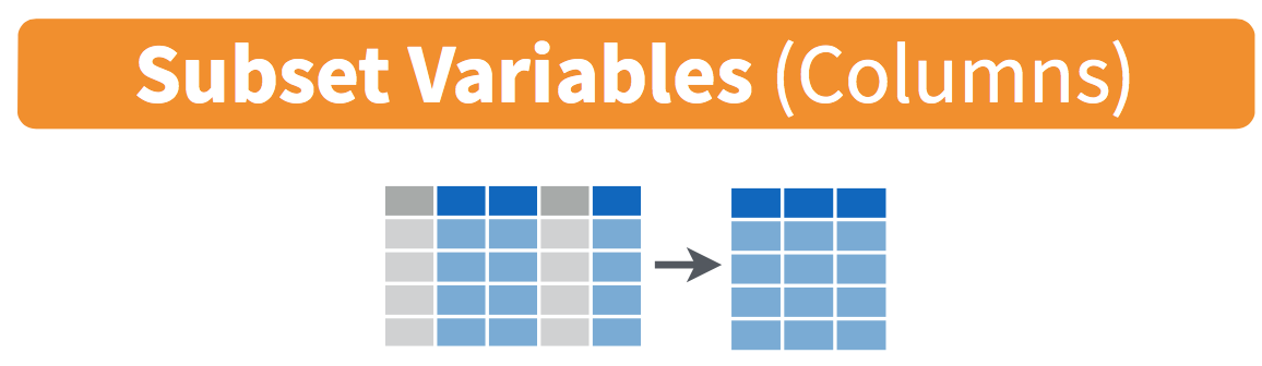
Figure 13.3: Select diagram from Data Wrangling with dplyr and tidyr cheatsheet
We’ve seen that the atlas data frame contains 62 different variables. You can identify the names of these 19 variables by running the glimpse() function from the dplyr package:
However, say you only need two of these variables, say state and emp2000. You can select() these two variables:
This function makes exploring data frames with a very large number of variables easier for humans to process by restricting consideration to only those we care about, like our example with state and emp2000 above. This might make viewing the dataset using the View() spreadsheet viewer more digestible. However, as far as the computer is concerned, it doesn’t care how many additional variables are in the data frame in question, so long as state and state are included.
Lastly, the helper functions starts_with(), ends_with(), and contains() can be used to select variables/column that match those conditions. For example:
13.4.2 rename variables
Another useful function is rename(), which as you may have guessed renames one column to another name. Suppose we want emp2000 and popdensity2010 to be employmentrate2000 and populationdensity2010 instead in the atlas data frame:
atlas <- atlas %>%
  rename(populationdensity2010 = popdensity2010,
         employmentrate2000 = emp2000)
glimpse(atlas)
Note that in this case we used a single = sign within the rename(). This is because we are not testing for equality like we would using ==, but instead we want to assign a new variable populationdensity2010 to have the same values as popdensity2010 and then delete the variable popdensity2010. It’s easy to forget if the new name comes before or after the equals sign. I usually remember this as “New Before, Old After” or NBOA.
13.4.3 top_n values of a variable
We can also return the top n values of a variable using the top_n() function. For example, we can return a data frame of the top neighborhoods by mobility for children from parents in the percentile 25. Observe that we set the number of values to return to n = 10 and wt = kfr_pooled_p25 to indicate that we want the rows of corresponding to the top 10 values of kfr_pooled_p25. See the help file for top_n() by running ?top_n for more information.
Let’s further arrange() these results in descending order of kfr_pooled_p25:
You can read more about the function arrange() here, but the logic is fairly simple. We are organizing the neighborhoods in descending order in the variable kfr_pooled_p25.
13.5 Conclusion
13.5.1 Additional resources
If you want to further unlock the power of the dplyr package for data wrangling, we suggest you that you check out RStudio’s “Data Transformation with dplyr” cheatsheet. This cheatsheet summarizes much more than what we’ve discussed in this chapter, in particular more-intermediate level and advanced data wrangling functions, while providing quick and easy to read visual descriptions.
You can access this cheatsheet by going to the RStudio Menu Bar -> Help -> Cheatsheets -> “Data Transformation with dplyr”:
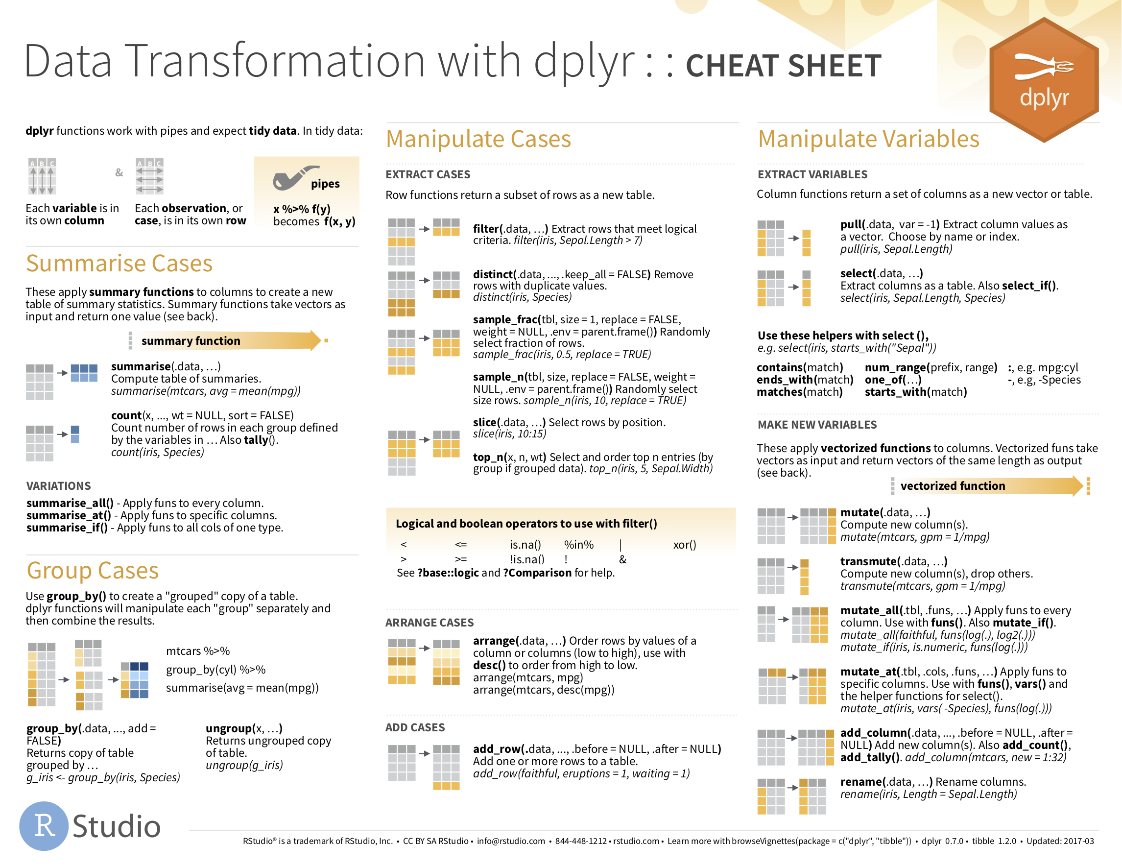
Figure 13.4: Data Transformation with dplyr cheatsheat
On top of data wrangling verbs and examples we presented in this section, if you’d like to see more examples of using the dplyr package for data wrangling check out Chapter 5 of Garrett Grolemund and Hadley Wickham’s and Garrett’s book (rds2016?).